
IEEE 802.15.4 Encoding
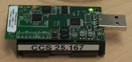
This is a walk through the encoding process of an IEEE 802.15.4 frame. It demonstrates the creation of the complex baseband signal that can be sent with a SDR to a sensor mote like this one.
msg = "Hello GNU Radio!\n"
We have to prepend the message with header information, which is defined in the IEEE 802.15.4 standard. You can download the standard for free from IEEE here.
In the first step, we create a MPDU out of the data payload.
import struct
from math import sin, pi
try:
    seqNr = (seqNr + 1) % 256
except:
    seqNr = 0

# crc calculation is a bit ugly
def crc(buf):
    c = 0
    bytes = struct.unpack("%dB" % len(buf), buf)
    for i in bytes:
        for k in range(8):
            b = (not(not((i & (1 << k)))) ^ (c & 1))
            c = c >> 1
            if(b):
                c ^= (1 << 15)
                c ^= (1 << 10)
                c ^= (1 <<  3)
    return struct.pack("BB", c & 0xFF, c >> 8)

# I hope from here on the code looks a bit nicer
def make_packet(payload):

    # I put some so-called RIME header in front of the payload
    # to ease interoperability with the real mote easier. The mote runs Contiki
    # and has an open RIME connection
    payload = struct.pack("BBBB", 0x81, 0x00, 0x2a, 0x17) + payload

    # we start with a known pattern that the mote is searching for
    start = struct.pack("BBBBB", 0x00, 0x00, 0x00, 0x00, 0xA7);

    # then there is a length field that tells the mote how long it
    # should try to decode (the overhead (11 bytes) is due to headers)
    length = struct.pack("B", len(payload) + 11)

    # tell the mote what type of frame we are sending (frame control)
    fc = struct.pack("BB", 0x41, 0x88)

    # a sequence number. We have to increment it, if we want to send
    # multiple packets. If we don't, the transceiver will silently
    # drop packets as it thinks they are duplicates
    seq = struct.pack("B", seqNr)

    # we put in some arbitrary addressing information
    # the allowed addressing formats are defined in the standard
    addr = struct.pack("BBBBBB", 0xcd, 0xab, 0xff, 0xff, 0x40, 0xe8)

    # assemble everything
    packet = start + length + fc + seq + addr + payload

    # calculate a checksum so that the mote can detect if
    # everything went right during transmission
    return packet + crc(packet[6:])

packet = make_packet(msg)
The packet is now a chunk of bytes. In hex representation it looks like this:
print map(lambda x: hex(ord(x)), packet[:10]).__repr__()
We split every byte of the packet into lower and upper nipple of 4 bits. The lower nipple is transmitted first.
def split_byte(b):
    return [ord(b) & 0xF, ord(b) >> 4]

nipples = map(split_byte, packet)
# now nipples is a list of lists with 2 values each
# we have to merge it
nipples = [j for i in nipples for j in i]
Now, we end up with a list, which is twice as long as the packet. Currently, it looks like this:
print map(hex, nipples[:10]).__repr__()
Note, how for example 0xa7 is split into 0x7, 0xa.
Every nipple is mapped to a 32 bit chip sequence. If you have the standard at hand, the sequences are defined in Section 6.5.2.3.
chips_sequences = [
    0b11011001110000110101001000101110,
    0b11101101100111000011010100100010,
    0b00101110110110011100001101010010,
    0b00100010111011011001110000110101,
    0b01010010001011101101100111000011,
    0b00110101001000101110110110011100,
    0b11000011010100100010111011011001,
    0b10011100001101010010001011101101,
    0b10001100100101100000011101111011,
    0b10111000110010010110000001110111,
    0b01111011100011001001011000000111,
    0b01110111101110001100100101100000,
    0b00000111011110111000110010010110,
    0b01100000011101111011100011001001,
    0b10010110000001110111101110001100,
    0b11001001011000000111011110111000
]

# the notation in the standard starts with the
# least significant bit. We have to mirror
# the binary representation
def mirror(n, bits):
    o = 0
    for i in range(bits):
        if(n & (1 << i)):
            o = o | (1 << (bits - 1 - i))
    return o

chips = map(lambda x: mirror(chips_sequences[x], 32), nipples)

print chips[:5].__repr__()
The chip sequences in the standard are given as $b_0 b_1 b_2\cdots$. With the mirror function we turn around the bit representation to $b_{31} b_{30} b_{29}\cdots$.
The chip sequences will get O-QPSK encoded, which is a slight variation of QPSK. QPSK defines 4 different constellations and thus, encodes 2 bits. For that reason we split every chip sequence in 2 bit chunks now.
def map_bits(b):
    ret = []
    for i in range(16):
        ret.append((b >> (i * 2)) & 3)
    return ret

bits = map(map_bits, chips)
# now bits is a list of lists. We
# make a big list out of it
bits = [j for i in bits for j in i]

# let's just look at some of the chunks
print bits[:20].__repr__()
OK, now we have the 2 bit blocks that we can map to QPSK constellations.
def map_symbols(b):
    if(b == 0):
        return -1 - 1j
    elif(b == 1):
        return  1 - 1j
    elif(b == 2):
        return -1 + 1j
    elif(b == 3):
        return  1 + 1j


syms = map(map_symbols, bits)

# things are getting complex :)
print syms[:10].__repr__()
We decide to send 4 samples per symbol (this is somehow arbitrary, we just have to assure that the sample rate is high enough so that the signal has a somewhat nice shape when it is emitted by the USRP). The standard mandates a chip bit rate of 2Mbit/s. A QPSK symbols encodes 2 bits and hence the symbols rate is 1Mbit/s. We just decided to transmit 4 samples per symbol and therefore, end up with a sample rate of 4Mbit/s. We keep that in mind as we later have to set the sample rate of the USRP accordingly. But for now, we just repeat each symbol 4 times.
Now, we apply a half sine pulse shape.
shaped_syms = map(lambda x: [x * k for k in [0, sin(pi/4), 1, sin(3*pi/4)]], syms)
# again, transform list of lists to a big list
shaped_syms = [j for i in shaped_syms for j in i]
# print
print [format(x, ".3") for x in shaped_syms[:5]]
%matplotlib inline import matplotlib.pyplot as plt plt.style.use('bmh') plt.rcParams['figure.facecolor'] = '#222222' plt.rcParams['axes.facecolor'] = 'None' plt.rcParams['figure.figsize'] = (10, 10.0*2/3) plt.rcParams['font.size'] = 14 plt.rcParams['lines.linewidth'] = '3'We can have a look at how the pulse shape smoothes the transitions between symbols.
%matplotlib inline
import matplotlib.pyplot as plt
plt.style.use('bmh')
plt.rcParams['figure.figsize']   = (10, 10.0*2/3)
plt.rcParams['font.size']        = 14
plt.rcParams['lines.linewidth']  = '3'

# this is an interpolated version of the signal
# where every symbol is repeated 4 times
interp_syms = map(lambda x: [x.real]*4, syms)
interp_syms = bits = [j for i in interp_syms for j in i]
plt.plot(interp_syms[:70])

# this is the shaped version that we just created
plt.plot(map(lambda x: x.real, shaped_syms[:70]))
plt.ylim([-1.1, 1.1]);

We use O-QPSK encoding, where we delay the quadrature component, i.e. the complex part of the symbol by half the symbol length (in our case 2 samples, as the symbol length is 4 samples). This is also done in order to make smoother transitions from one symbol to the other. On the one hand, we now have twice as much switches (transitions) however, on the other hand, we never switch both inphase and quadrature components at the same time. In other words, we trade more transitions for smoother transitions.
real = map(lambda x: x.real, shaped_syms)
imag = map(lambda x: x.imag, shaped_syms)

# shift I and Q relative to each other
# by 2 samples
real = real + [0, 0]
imag = [0, 0] + imag

# sum up the two shifted components. Real and imaginary, i.e. inphase and
# quadrature components.
signal = [a + b for a, b in zip(map(complex, real), map(lambda x: 1j*x, imag))]
# print
print [format(x, ".3") for x in signal[:5]]
aaaaaand we're done!
We can now send the complex baseband samples with a USRP. To accomplish this, we store the samples in a file that GNU Radio can read. We also pad the actual signal with some zeros.
import numpy as np

filename = "/tmp/sensor.raw"

#write_signal = 1000000 * [complex(0)] + signal + 1000000 * [complex(0)]

#np_sig = np.array(write_signal, dtype=np.complex64)
#np_sig.tofile(filename)
Now you have several options how to transmit that file:
- You can use the tx_samples_from_file that is included in the UHD library.
- You can create a simple flow graph that reads from a file and transmits the samples.
- You can use that file as input of the rx chain included in the examples folder. In that case, you have to replace the USRP source block with a file source and a rational resampler and sample it up by 2.5 (decimation 4, interpolation 10).
The most interactive approach is to write the data to a pipe, where the tx_samples_from_file program is reading from. Then your packet is transmitted instantly when you write to the pipe (i.e. run this notebook). Thus, you can transmit a frame directly from your browser.
The following script might help to setup a pipe in Linux.
#!/bin/bash

FILE="/tmp/sensor.raw"
rm -i ${FILE}

TX_APP="/usr/local/lib/uhd/examples/tx_samples_from_file"
GAIN="30"
FREQ=2480000000
SAMPLES_PER_BURST=500
RATE=4000000

### create fifo
if [ -e ${FILE} ]
then
    echo "${FILE}: file already exists"
    if ! [ -p ${FILE} ]
    then
        echo "WARNING: ${FILE} is not a FIFO"
    fi
else
    echo "creating fifo ${FILE}"
    mkfifo ${FILE}
fi

### start TX
${TX_APP}   --file ${FILE}\
            --type float\
            --spb ${SAMPLES_PER_BURST}\
            --rate ${RATE}\
            --freq ${FREQ}\
            --gain ${GAIN}
Finally, we can have a look at the signal in time domain:
plt.plot(map(lambda x: x.real, signal[:100]))
plt.plot(map(lambda x: x.imag, signal[:100]));

...and in frequency domain:
fft_size = 2048
freq = np.fft.fftshift(np.fft.fft(signal[:fft_size]))
x = np.linspace(-4e6/2, 4e6/2, len(freq))

fig, ax = plt.subplots()
ax.set_xticks([-2e6, -1e6, 0, 1e6, 2e6])
ax.plot(x, abs(freq));
